Stability of steady-state equilibrium for overlapping generation model
This is a summary of discussion with Alecos Papadopoulos at http://economics.stackexchange.com/questions/16118/stability-of-steady-state-equilibrium-for-overlapping-generation-model as well as from what I learnt and thought in my graduate macroeconomics class.
Draft version. You are welcome to go to http://economics.stackexchange.com/questions/16118/stability-of-steady-state-equilibrium-for-overlapping-generation-model to comment and answer.
- In draft edition of Daron Acemoglu's Introduction to Modern Economic Growth (2007), proposition 9.4 which states that:
In the overlapping-generations model with two-period lived households, Cobb-Douglas technology and CRRA preferences, there exists a unique steady-state equilibrium with the capital-labor ratio k* given by (9.15) and as long as $\theta \geq 1$
has a typo. In 2009 edition of the textbook, proposition 9.4 is corrected to:, this steady-state equilibrium is globally stable for all k (0) > 0.
In the overlapping-generations model with two-period lived households, Cobb-Douglas technology and CRRA preferences, there exists a unique steady-state equilibrium with the capital-labor ratio k* given by (9.15) and for any $\theta$ > 0
, this steady-state equilibrium is globally stable for all k (0) > 0.
-
In the following, we will use the setup and symbol of overlapping-generations model with two-period lived households, Cobb-Douglas technology and CRRA preferences as in Daron Acemoglu's Introduction to Modern Economic Growth (2009).
To show $\theta > 0$ is the condition for stable steady-state equilibrium for overlapping generation model, we use formula (9.17) derived in the textbook:
$$k(t+1)=\frac{(1-\alpha)k(t)^\alpha}{(1+n)[1+\beta^{-\frac{1}{\theta}}(\alpha k(t+1)^{\alpha-1})^{\frac{\theta-1}{\theta}}]}$$
We can rearrange to get:
$$
k(t)=\big[ \frac{1+n}{1-\alpha} [k(t+1)+\beta^{-\frac{1}{\theta}}\alpha^{\frac{\theta-1}{\theta}}k(t+1)^{(\alpha-1)(1-\frac{1}{\theta})+1}] \big]^\frac{1}{\alpha} \text{ .....(1)}
$$
-
Case $\theta = 0$:Note that when the textbook derives (9.17), it implicitly assumes that $\theta \neq 0$ (for derivation of Euler equation for consumption in P.333 of 2009 edition of the textbook). When $\theta = 0$, equation (1) no longer applies. Returning to the utility maximization problem with $\theta = 0$: $$ \text{max } U(t) = c_1(t) + \beta(c_2(t+1)) \text{ such that } c_1(t) + \frac{c_2(t+1)}{R(t+1)} = w(t) \\ \Leftrightarrow \text{max } U(t) = c_1(t) + \beta(w(t) - c_1(t))R(t+1) $$
- Wrong version (Treat utility maximization problem as central-planner problem):$$ \text{max } U(t) = c_1(t) + \beta(w(t) - c_1(t))R(t+1) \\ = c_1(t) + \beta(w(t) - c_1(t))f'(k(t+1)) \text{ ...Wrong to set $R(t+1) = f'(k(t+1))$, treating it as central-planner problem} \\ = c_1(t) + \beta(w(t) - c_1(t))\alpha k(t+1)^{\alpha - 1} \\ = c_1(t) + \beta(w(t) - c_1(t))\alpha (\frac{s(t)}{1+n})^{\alpha - 1} \text{ (Given full capital depreciation)}\\ = c_1(t) + \beta s(t) \alpha (\frac{s(t)}{1+n})^{\alpha - 1} \\ = w(t) - s(t) + \frac{\alpha\beta}{(1+n)^{\alpha - 1}} s(t)^\alpha \\ $$ First-order condition with respect to $s(t)$ gives: $$ s(t)^* = (1+n)(\alpha^2 \beta)^{\frac{1}{1 - \alpha}} $$ Then, $$ k(t+1) = \frac{s(t)}{1+n} = (\alpha^2 \beta)^{\frac{1}{1 - \alpha}}\text{ , which is a constant} $$ This means that the steady-state equilibrium where $k^* = (\alpha^2 \beta)^{\frac{1}{1 - \alpha}}$ is globally stable as even k deviates from $k^*$ for one period, next period k will return to steady state $k^*$.
-
Correct version (To be confirmed):$$ \text{max } U(t) = c_1(t) + \beta(w(t) - c_1(t))R(t+1) \\ = c_1(t) (1 - \beta R(t+1)) + \beta R(t+1)w(t) \text{ ...Should treat R(t+1) as given as consumer's own optimization problem}\\ $$ s(t) has to be non-negative for $k(t+1)= \frac{s(t)}{1+n}$ and k(t+1) is non-negative. $$ c_1(t)^* = \begin{cases} w(t)\text{, for }\beta R(t+1) <1 \\ [0, w(t)]\text{, for }\beta R(t+1) = 1 \\ 0\text{, for }\beta R(t+1) > 1 \\ \end{cases} $$ $$ s(t)^* = \begin{cases} 0\text{, for }\beta R(t+1) <1 \\ w(t) - c_1(t)^* \in [0, w(t)]\text{, for }\beta R(t+1) = 1 \\ w(t)\text{, for }\beta R(t+1) > 1 \\ \end{cases} $$ For $R(t+1) = f'(k(t+1)) = \alpha k(t+1)^{\alpha - 1}$, $$ k(t+1) = \frac{s(t)}{1+n} = \begin{cases} 0\text{, for }\beta R(t+1) <1 \Leftrightarrow k(t+1) < (\alpha \beta)^{\frac{1}{1 - \alpha}} \\ \frac{w(t) - c_1(t)}{1+n} \in [0, \frac{w(t)}{1+n}]\text{, for }\beta R(t+1) = 1 \Leftrightarrow k(t+1) = (\alpha \beta)^{\frac{1}{1 - \alpha}}\\ \frac{w(t)}{1+n} = \frac{k(t)^\alpha - k(t)\alpha k(t)^{\alpha -1}}{1+n} = \frac{1-\alpha}{1+n}k(t)^\alpha\text{, otherwise} \Leftrightarrow k(t) > [\frac{1+n}{1 - \alpha} (\alpha \beta)^{\frac{1}{1 - \alpha}}]^{\frac{1}{\alpha}} \\ \end{cases} $$
-
Original wrong derivation:From this, we can draw the following graph:
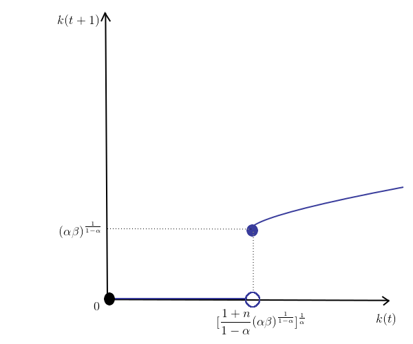
The blue line is: $$ k(t+1) = \begin{cases} \frac{1-\alpha}{1+n}k(t)^\alpha\text{, for }k(t) \geq [\frac{1+n}{1 - \alpha} (\alpha \beta)^{\frac{1}{1 - \alpha}}]^{\frac{1}{\alpha}} \\ 0\text{, otherwise} \end{cases} $$ For $\frac{1-\alpha}{1+n} k(t)^\alpha = k(t)$, $k(t) = [\frac{1-\alpha}{1+n}]^{\frac{1}{1-\alpha}}$ i.e. blue line crosses the 45-degress line when $k(t) = [\frac{1-\alpha}{1+n}]^{\frac{1}{1-\alpha}}$. $$ D = [\frac{1+n}{1 - \alpha} (\alpha \beta)^{\frac{1}{1 - \alpha}}]^{\frac{1}{\alpha}} - [\frac{1-\alpha}{1+n}]^{\frac{1}{1-\alpha}} \\ = \frac{1+n}{1-\alpha}^{\frac{1}{\alpha}}[(\alpha \beta)^{\frac{1}{\alpha (1-\alpha)}} - (\frac{1+n}{1-\alpha})^{\frac{-1}{(1-\alpha)\alpha}}] $$- Case 1: $D > 0 \Leftrightarrow \alpha > \frac{1}{1+(1+n)\beta}$
We can draw the following graph:
 The red line is 45-degrees line. It can be seen that for all $k > 0$, k will converge to steady-state S k* = 0. The steady-state equilibrium is globally stable.
- Case 2: $D = 0 \Leftrightarrow \alpha = \frac{1}{1+(1+n)\beta}$
We can draw the following graph:
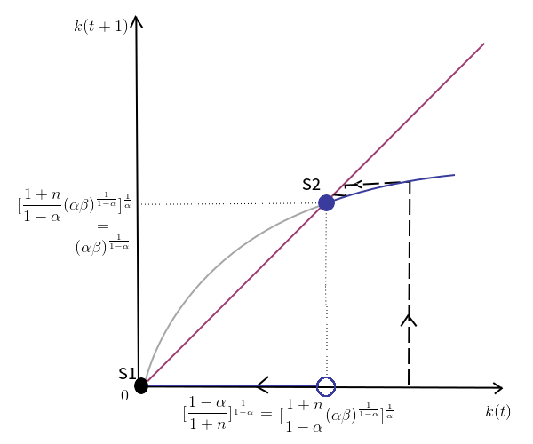 The red line is 45-degrees line. It can be seen that for all $0 < k < [\frac{1-\alpha}{1+n}]^{\frac{1}{1-\alpha}}$, k will converge to steady-state S1 k* = 0 while for all $k \geq [\frac{1-\alpha}{1+n}]^{\frac{1}{1-\alpha}}$, k will converge to steady-state S2 k* = $(\alpha \beta)^{\frac{1}{1-\alpha}}$. The steady-state equilibria are not globally stable.
- Case 3: $D < 0 \Leftrightarrow \alpha < \frac{1}{1+(1+n)\beta}$
We can draw the following graph:
 The red line is 45-degrees line. It can be seen that for all $0 < k < [\frac{1+n}{1 - \alpha} (\alpha \beta)^{\frac{1}{1 - \alpha}}]^{\frac{1}{\alpha}}$, k will converge to steady-state S1 k* = 0 while for all $k \geq [\frac{1+n}{1 - \alpha} (\alpha \beta)^{\frac{1}{1 - \alpha}}]^{\frac{1}{\alpha}}$, k will converge to steady-state S2 k* = $[\frac{1-\alpha}{1+n}]^{\frac{1}{1-\alpha}}$. The steady-state equilibria are not globally stable.
- Case 1: $D > 0 \Leftrightarrow \alpha > \frac{1}{1+(1+n)\beta}$
We can draw the following graph:
-
Correct derivation:
- Case 1: $\beta R(t+1) < 1 \Leftrightarrow R(t+1) < \frac{1}{\beta}$: As the production function $f(k)$ is Cobb-Douglas, it satisfies the Inada condition: $lim_{k(t) \to 0} f'(k(t)) = \infty$. But as $f'(k(t)) = R(t)$, $lim_{k(t) \to 0} R(t) < \infty$ for $R(t) < \frac{1}{\beta} < \infty$ as $\beta \in (0,1)$, violating the Inada condition. This contradiction means this case is impossible.
- Case 2: $\beta R(t+1) = 1 \Leftrightarrow \beta \alpha k(t+1)^{\alpha-1} = 1 \Leftrightarrow k(t+1)^{\alpha-1} = \frac{1}{\alpha \beta} \Leftrightarrow k(t+1)^{1-\alpha} = \alpha \beta$: Denote saving rate at t as $\mathcal{S}(t) = \frac{s(t)}{w(t)}$. $k(t+1) = \frac{s(t)}{1+n} = \frac{\mathcal{S}(t)w(t)}{1+n} = \frac{\mathcal{S}(t)(1-\alpha)k(t)^\alpha}{1+n}$. At steady state, $k^* = \frac{\mathcal{S}^*(1-\alpha){k^*}^\alpha}{1+n}$, meaning $\mathcal{S}^* = \frac{1+n}{1-\alpha}{k^*}^{1-\alpha} = \frac{1+n}{1-\alpha} \alpha \beta$. For $\mathcal{S}^* > 1 \Leftrightarrow (1+n)\alpha\beta > 1 - \alpha \Leftrightarrow \beta > \frac{1 - \alpha}{\alpha (1+n)}$, which is possible. As saving rate cannot be larger than 1, this contradiction means this case is impossible.
- Case 3: $\beta R(t+1) > 1$:
This case is possible.
$$
k(t+1) = \frac{1-\alpha}{1+n} k(t)^\alpha
$$
We can draw the graph:
The red line is 45-degrees line. The blue line is $k(t+1) = \frac{1-\alpha}{1+n} k(t)^\alpha$ where $0 < \alpha < 1$. For all k(0) > 0, k will converge to steady state $k^* = \frac{1-\alpha}{1+n} {k^*}^\alpha \Leftrightarrow k^* = [\frac{1-\alpha}{1+n}]^{\frac{1}{1-\alpha}}$. The steady-state equilibrium is globally stable.
 TODO: investigate why proposition in textbook not relax the condition of globally stable steady-state equilibrium to $\theta \geq 0$
-
-
-
Case $\theta > 0$:
- Informal way:
Let $n = 0.01$, $\alpha = 0.25$, $\beta = 0.75$.
If $\theta > 0$, we can plot a graph like this$^{[1]}$:
The blue line is equation (1) where $\theta = 1$ and the red line is 45-degrees line. It can be seen that for all k > 0, k will converge to steady-state k*. The steady-state equilibrium is globally stable.
- Informal way:
Let $n = 0.01$, $\alpha = 0.25$, $\beta = 0.75$.
-
Case $\theta < 0$:
- Informal way:
Let $n = 0.01$, $\alpha = 0.25$, $\beta = 0.75$.
If $\theta < 0$, we can plot a graph like this$^{[1]}$:
The blue line is equation (1) where $\theta = -1$ and the red line is 45-degrees line. It can be seen that for some k > 0, k will not converge to steady-state k*. The steady-state equilibrium is not globally stable.
- Informal way:
Let $n = 0.01$, $\alpha = 0.25$, $\beta = 0.75$.
-
- TODO: discuss intuition
- Formal proof of the proposition can be found in Michael Peters and Alp Simsek's Solutions Manual for "Introduction to Modern Economic Growth" - Answer for Exercise 9.6.
- Acknowledgement: [1] The graphs are modified from those generated by Wolframalpha.

Comments
Post a Comment